Groundwater
Aquifer modelling, in 1D and under the 2D surface
Where the water table sits near the ground, the ground stops soaking up rain and low areas flood deeper. AquaSWMM models that with SWMM's two-zone aquifer: in 1D on EPA's own engine, and in 2D under every cell of the surface grid. The 2D version adds infiltration into pipes and seepage back onto low ground, and its water balance closes to round-off.
The model: two zones, one water table
Each aquifer is SWMM's lumped two-zone store (Rossman & Huber 2016, SWMM Reference Manual Vol. I: Hydrology, ch. 5): an unsaturated upper zone with a uniform moisture content θ, over a saturated lower zone of depth dL. The flux laws and the integrator are EPA's own. In 2D, the cells above an aquifer feed it with the infiltration they compute, and it drains to a network node exactly as a SWMM subcatchment's aquifer does.
ddL/dt = (fU − eL − fL − fG − fGWI − fS) / (φ − θ)
D = depth from the aquifer bottom to the ground surface; φ = porosity. Integrated with the fifth-order Cash–Karp Runge–Kutta scheme and SWMM's adaptive step control (tolerance 10−4).
| Flux | What it is | Formula |
|---|---|---|
| fI | Infiltration from the surface | From the infiltration method (Green–Ampt, Horton or constant loss), computed per 2D cell |
| eU | Upper-zone evapotranspiration | Upper ET fraction × potential ET, limited to what is left; none while infiltration occurs or below the wilting point |
| eL | Lower-zone evapotranspiration | (ET depth − upper-zone depth) / ET depth × (1 − upper fraction) × potential ET |
| fU | Percolation, upper to lower zone | Ks e−HCO(φ−θ) (1 + HCU · 2(θ − FC) / (D − dL)), when θ > field capacity |
| fL | Deep percolation | Seepage coefficient × dL / D, or a [GWF] DEEP expression |
| fG | Lateral flow to the node | A1(Hgw − H*)B1 − A2(Hsw − H*)B2 + A3 Hgw Hsw, plus an optional [GWF] LATERAL expression |
| fGWIAquaSWMM | Infiltration into sewer pipes | Σ C · πDp · L · max(0, Hwt − zinvert) over pipes below the water table |
| fSAquaSWMM | Seepage onto the surface | Ks over the 2D cells whose ground is at or below the water table; the water rejoins the 2D flow |
Hgw = water table above the aquifer bottom; Hsw = water level at the node; H* = threshold height; Ks = saturated conductivity; HCO, HCU = SWMM's conductivity and tension slopes; FC = field capacity.
Conservation by construction. SWMM books lateral flow by the trapezoid of its end-of-step rates and clamps its states, so its report carries a small groundwater continuity error. Under the 2D grid every flux is booked once, as the volume actually delivered, and after each step the lower-zone depth is solved so the store holds exactly what the books say. The network receives exactly what the aquifer gave up.
Under the 2D surface: Hurricane Ian, Winter Springs FL
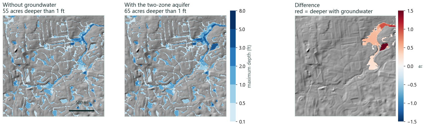
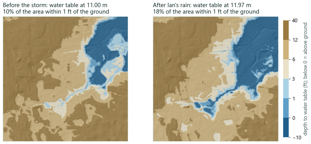
A 2 km square of Winter Springs on the USGS 3DEP 10 m DEM, forced by NOAA MRMS radar rain for Hurricane Ian (13.7 in, peak 3.0 in/hr), built by AquaSWMM's Storm Replay and run twice with Green–Ampt infiltration: once without groundwater and once over a sandy two-zone aquifer with its water table starting 3.4 m above the lowest ground. The aquifer parameters are illustrative Florida sand, not calibrated to a site.
| Groundwater balance, whole run | m³ |
|---|---|
| Infiltrated into the aquifer from the 2D cells | 1,163,386 |
| Seeped back onto low ground | 349,939 |
| Lateral flow to the outfall node | 46,043 |
| Change in storage | 767,404 |
| Balance error | −2.72×10⁻¹² % |
In 1D: EPA's engine, unmodified
EPA's Groundwater_Model sample (a 5-acre pervious subcatchment over a two-zone aquifer) with a pond added, driven by the same Ian rain and run on EPA SWMM 5.2.4 through AquaSWMM. The water table climbs from 3.51 ft to 4.85 ft, groundwater keeps feeding the pond after the rain stops, and the pond peaks at 3.0 ft.
Rain, water table and pond depth
Hourly values from the SWMM results file. Move across the chart to read all three at once.
- rain
- water table
- pond depth
Turning it on
- 1D: add an aquifer in the project browser (Hydrology → Aquifers) and give the subcatchment its groundwater parameters, as in EPA SWMM. The model stays a standard
.inp. - 2D: 2D → 2D Setup… → Groundwater: switch it on; cells take the aquifer of the subcatchment that owns them, with a default aquifer and receiving node for the rest; set the pipe-infiltration coefficient and seepage onto the surface.
- Results: the 2D layer picker's Water table depth overlay, the groundwater summary in the run log, and a groundwater results file for scripting.
- Start state: each run saves the aquifer state at its end, and the next run can start from that file.
[GROUNDWATER]
ON
STEP     60
SEEPAGE  YES
GWI      0
; aquifer  node  store  A1      B1   A2 B2 A3  fixed
DEFAULT FL_SAND O1  *   0.0001  1.5  0  0  0   0
The 2D settings live in a sidecar file beside the model, so the .inp still opens in EPA's GUI. In Python, pip install aquaswmm runs the same models and reads the groundwater results.
What it is not
- Lumped, not distributed. One water table per aquifer store. Groundwater does not flow sideways between stores or cells; there is no Darcy flow across the grid. It is SWMM's two-zone model, not a MODFLOW-type groundwater model.
- The Winter Springs aquifer parameters are illustrative. For design, calibrate them to boring logs and observed water tables.
- The 2D surface results are checked against analytic solutions and benchmarks, not yet against a measured real-world flood (see Validation).